Hi @skipburrows, you have two issues going on:
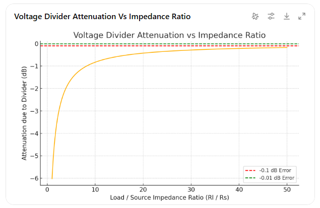
The first issue is loading as @Claudio and @restorer-john have pointed out. Below is a table that shows the ratio of DUT input Z to Generator Output Z. And that gives you a correction factor you can enter. For example, in balanced mode, the QA403 output Z is 200 ohms. If your DUT is 2k, then that’s a 10X ratio (2k/200), and you can compute or read from the chart that’s -0.827 dB. So, you can enter into the QA403 software the Output Gain of -0.827, and that will INCREASE the output gain of the analyzer by 0.827 dB to compensate for the divider losses. If you are also using balance mode output gain of 6.02 dB, then just add them and enter the sum of 6.02 - 0.827 = 5.193 dB.
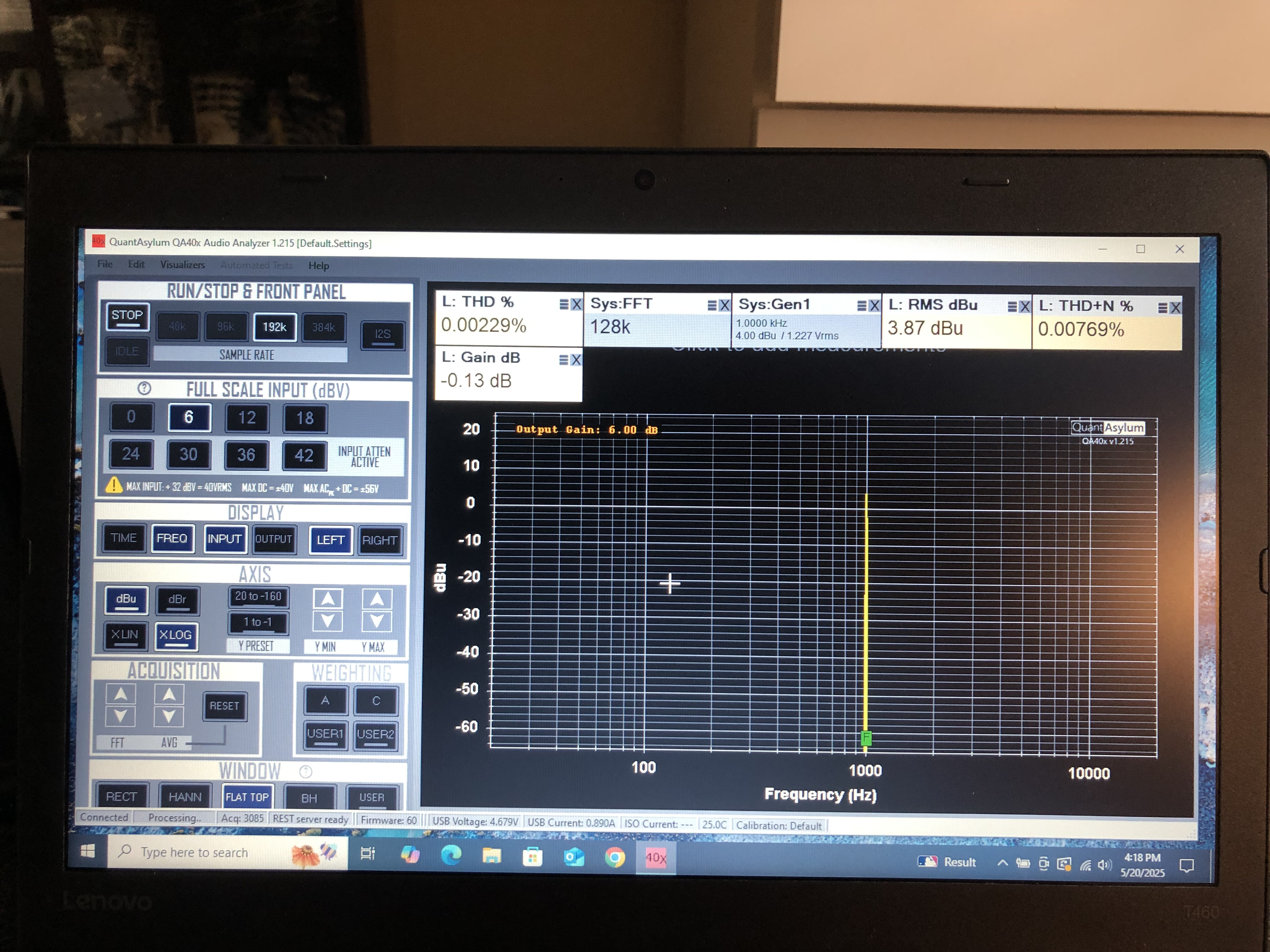
The second issue is very likely a transient issue. I hate to say it again, but you need to be provide the TIME DOMAIN plot. When you pasted your Fig 2.0, you just needed to push the TIME button and that would have given the info required to diagnose.
Measuring a Compressor
(See also HERE)
Below is the time domain of a guitar compressor output with the settings dialed in to exaggerate the visuals. You can clearly see the attack phase lasting almost 200 mS. Note the short 8k FFT, which is also contributing to the issue.
If we go to Settings and set Show Truncated Burst in Time Domain, the time domain plot will change to show us just the portion of the waveform that is being used for the FFT
And here’s the resulting plot. Note the burst upon which the FFT analysis is occurring isn’t uniform. That is a problem, because for an FFT to really make sense, you want the amplitude of the waveform to be constant. Note, too, that the RMS is reported at -26.26 dBV.
So, how do we fix this? Go back to this plot and notice that while the attack is nearly 200 mS in duration, we never really see the waveform hit its steady state. It looks like it just shy of 200 mS. But we might guess that it’ll be 400 mS to hit steady state.
So, knowing that, we can adjust the latency compensation so be more than 400 mS. What this is telling the system is “The first 400 mS of the burst will be chaotic. So, ignore it”
Now, with Show Truncated Burst off we see the full burst. And very clearly we can see that indeed we’re hitting steady state probably around 300 mS. And so our assumption of 400mS was good.
Next, let’s go back to show the truncated burst and then zoom in on that. And look at that! Our amplitude is rock solid throughout the burst!
And note, too, that the RMS has changed from -26.26 and dropped to -26.61 dBV. This is because in the first plot above (not constant envelope) we saw the attack artificially increasing the energy. But you could also have an attack artificially decreasing the energy. But the point is this: If you don’t have a constant envelope, you can readily see half a dB of measurement error either way.
So, when looking at dynamic signals, you need to spend a bit of time in the time domain to make sure you are feeding the FFT with data that makes sense. If you aren’t, measurement errors can creep in. You have the tools to to readily tailor the measurements to account for very dynamic signals. A compressor is very easy to measure by looking at the time domain and adjusting the latency comp accordingly. And once that is correctly set, you can move back to the frequency domain confident with the result you are seeing.